[Study Note] Privacy-Preserving Record Linkage (PPRL) & ML Attacks

What is Privacy-Preserving Record Linkage? (PPRL)

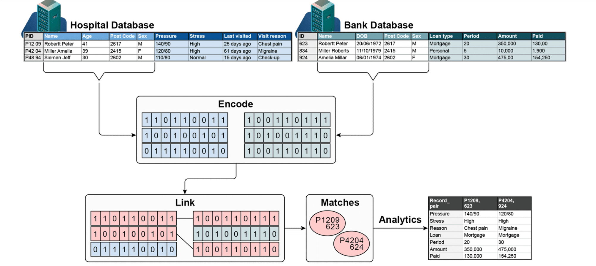
PPRL is a technique for matching records about the same individuals across different databases — without exposing their private data.

How it works

1. Two separate databases exist

• A Hospital DB with patient info (name, age, pressure, etc.)
• A Bank DB with financial info (name, DOB, loan type, etc.)

2. Encode

Instead of sharing raw personal data, each database converts its records into binary vectors (0s and 1s) using a technique like Bloom filters. The actual names/details are never directly shared.

3. Link

The encoded vectors from both databases are compared against each other to find similar patterns.

4. Matches

Records that are sufficiently similar are identified as referring to the same person (e.g., P1209 (hospital) = 623 (bank)).

5. Analytics

Once matched, the combined data can be used for analysis — without either party ever seeing the other’s raw records.

Why it matters

The key privacy guarantee is that neither database sees the other’s sensitive information. Only the encoded representations are exchanged, protecting individual privacy while still enabling useful data integration.

---

Application of PPRL

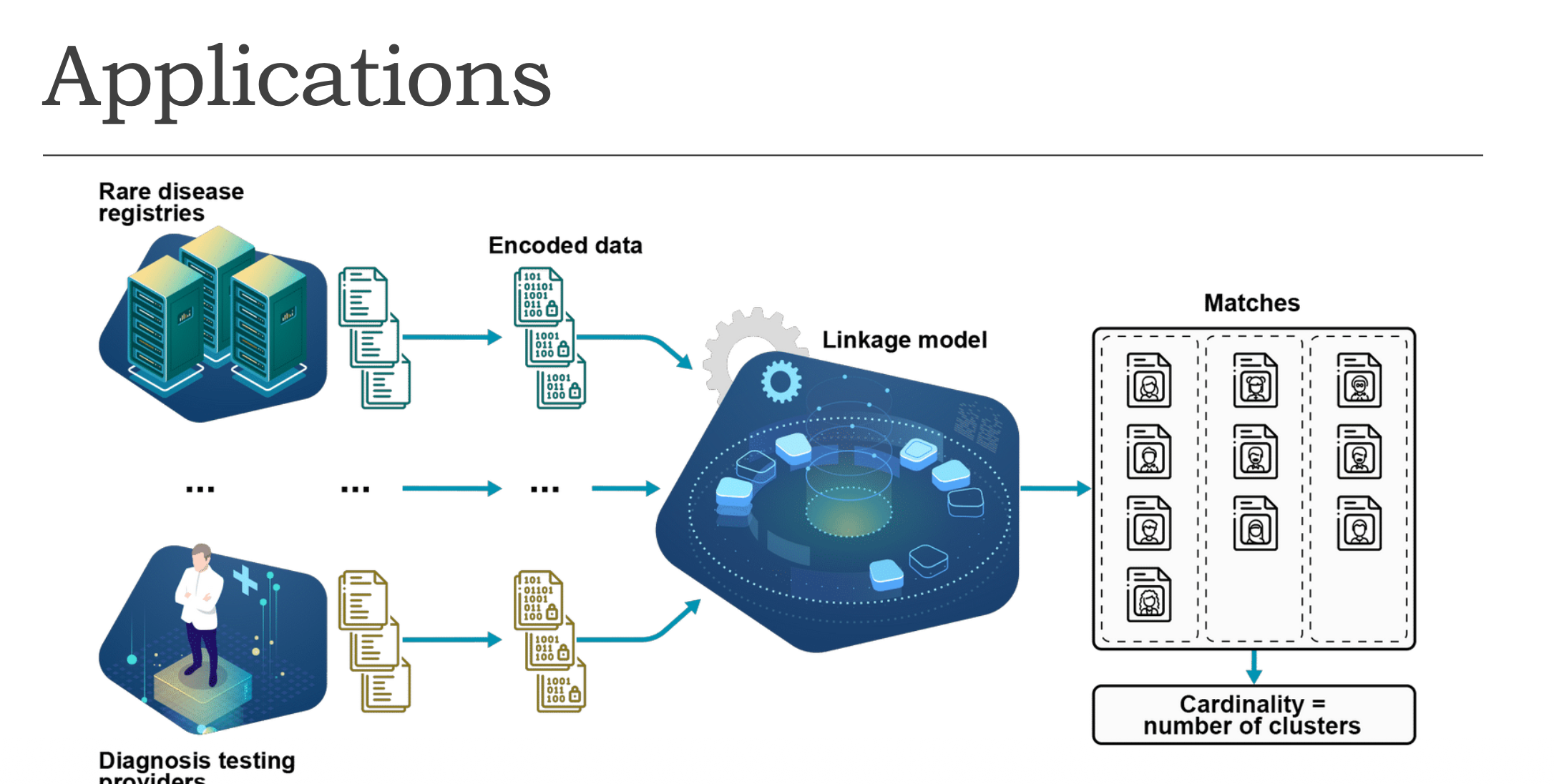
A real-world application in the healthcare domain:

① Two data sources

• Rare disease registries — databases storing records of patients with rare diseases
• Diagnosis testing providers — organisations that conduct medical tests

② Encoding

Both sources convert their raw records into encoded (binary) data before sharing.

③ Linkage Model

All encoded data flows into a central linkage model that compares records across multiple sources.

④ Matches & Clustering

The model groups matched records into clusters — each cluster represents one unique individual. Cardinality = number of clusters (total count of distinct individuals identified).

---

Key Challenges

1. Privacy
2. Linkage quality
3. Computational efficiency

---

PPRL Pipeline

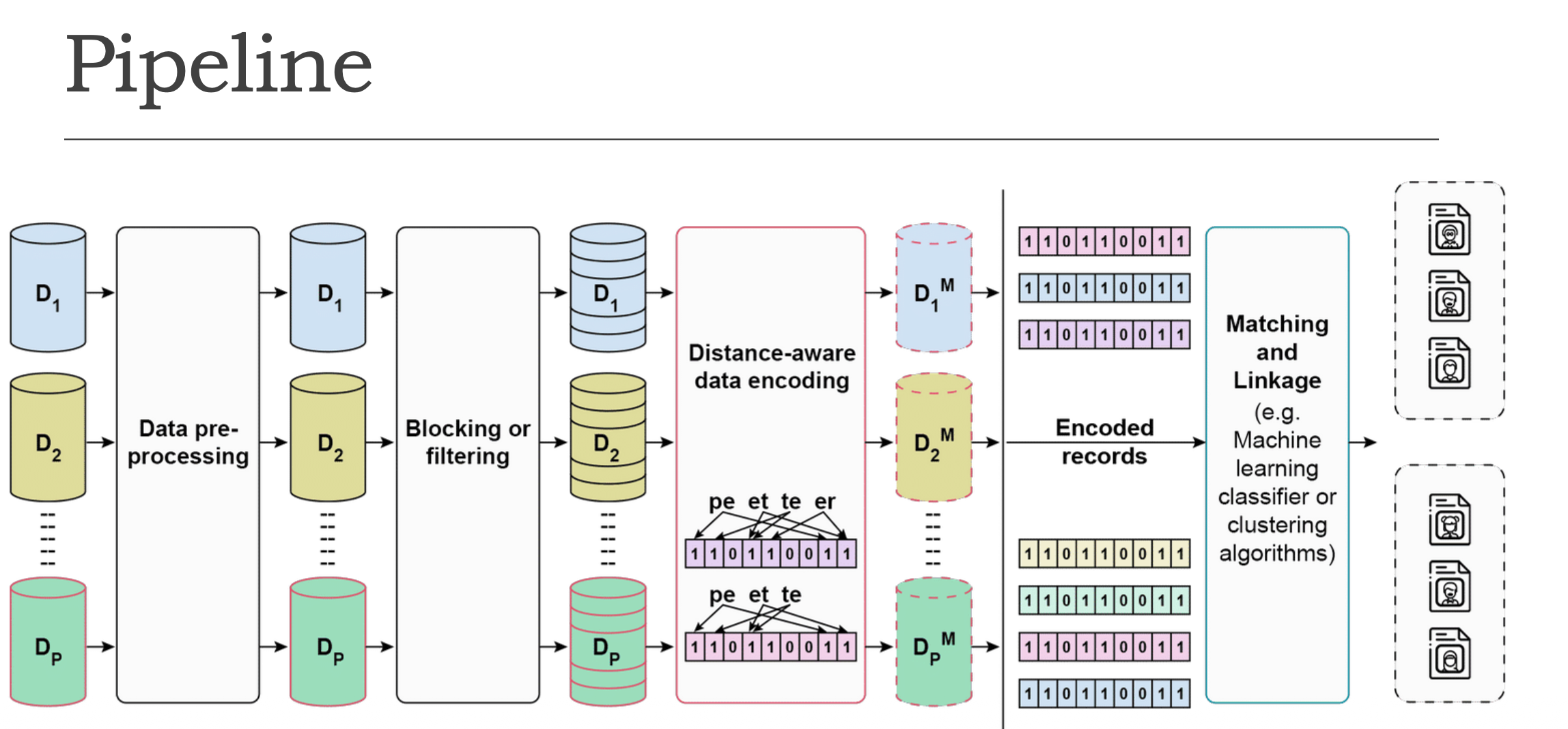
① Multiple Databases (D₁, D₂, … Dₚ) — Several databases from different organisations, each holding raw sensitive personal data.

② Data Pre-processing — Raw data is cleaned and standardised (e.g., fixing typos, formatting names/dates consistently).

③ Blocking or Filtering — Reduces the number of record pairs that need to be compared. Only records that are likely matches are kept.

④ Distance-aware Data Encoding (the key step)

Records are converted into binary vectors (0s and 1s). The encoding preserves similarity — similar records in real life will have similar binary vectors, making them candidates worth comparing more closely.

e.g., “peter” → bigrams (pe, et, te, er) → mapped into a bit vector

⑤ Encoded Records (D₁ᴹ, D₂ᴹ, … Dₚᴹ) — All databases now hold only encoded versions of their data.

⑥ Matching and Linkage — Encoded records are compared using ML classifiers or clustering algorithms.

⑦ Output — Clusters — Final result: groups of matched records, each cluster representing one unique individual.

---

Blocking

Why do we need Blocking?

When linking two databases, you’d normally compare every record against every other record — this is quadratic complexity. If each database has 1,000 records, you’d need 1,000,000 comparisons. That’s extremely slow and inefficient!

What is Blocking?

Blocking is a filtering step that groups records into smaller buckets called blocks, so you only compare records within the same block.

Example — Postcode as a Blocking Key

Record	Name	Postcode
A	John Smith	2000
B	Jane Doe	3000
C	Jon Smyth	2000

• Records A and C → same block (postcode 2000) → compared ✅
• Records A and B → different blocks → skipped ❌

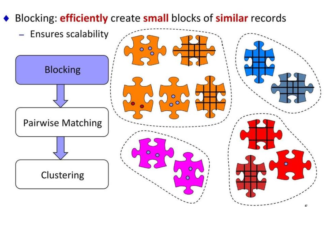
Each colour in the puzzle represents a block — only pieces of the same colour get compared.

After Blocking

Blocking → Pairwise Matching → Clustering

Blocking dramatically reduces the number of comparisons needed, making the whole linkage process fast and scalable.

---

Data Encoding: Exact Matching Using Bloom Filters

What is a Bloom Filter?

A Bloom filter is a bit vector (a row of 0s and 1s) that represents a piece of data. Each value gets mapped to specific positions in the vector.

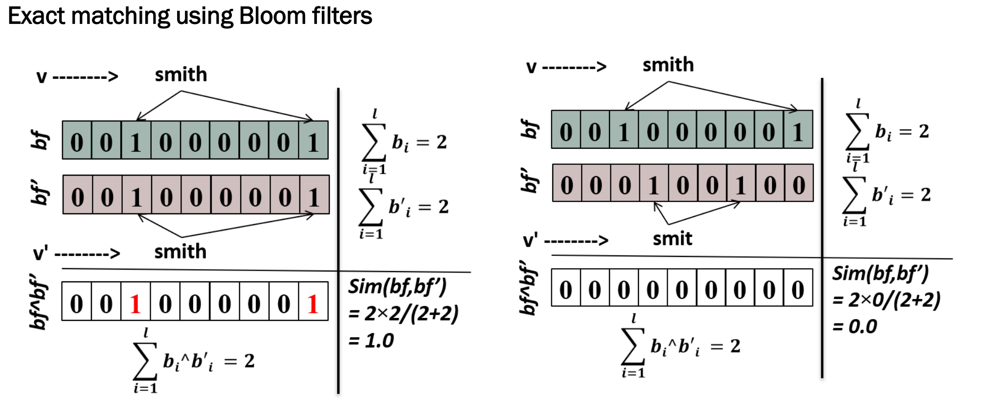
Example: “smith” vs “smith” (identical)

bf  = 0 0 1 0 0 0 0 0 1   (smith)
bf' = 0 0 1 0 0 0 0 0 1   (smith)

AND: 0 0 1 0 0 0 0 0 1  →  matching bits = 2

Sim = 2 × 2 / (2 + 2) = 1.0  ✅ Perfect match!

Example: “smith” vs “smit” (different)

bf  = 0 0 1 0 0 0 0 0 1   (smith)
bf' = 0 0 0 1 0 0 1 0 0   (smit)

AND: 0 0 0 0 0 0 0 0 0  →  matching bits = 0

Sim = 2 × 0 / (2 + 2) = 0.0  ❌ No match!

The Similarity Formula (Dice Coefficient)

\[Sim(bf, bf') = \frac{2 \times |bf \wedge bf'|}{|bf| + |bf'|}\]

This is called exact matching — even a tiny difference (e.g. “smith” vs “smit”) results in a similarity score of 0.0.

---

Data Encoding: Fuzzy Matching Using Bloom Filters

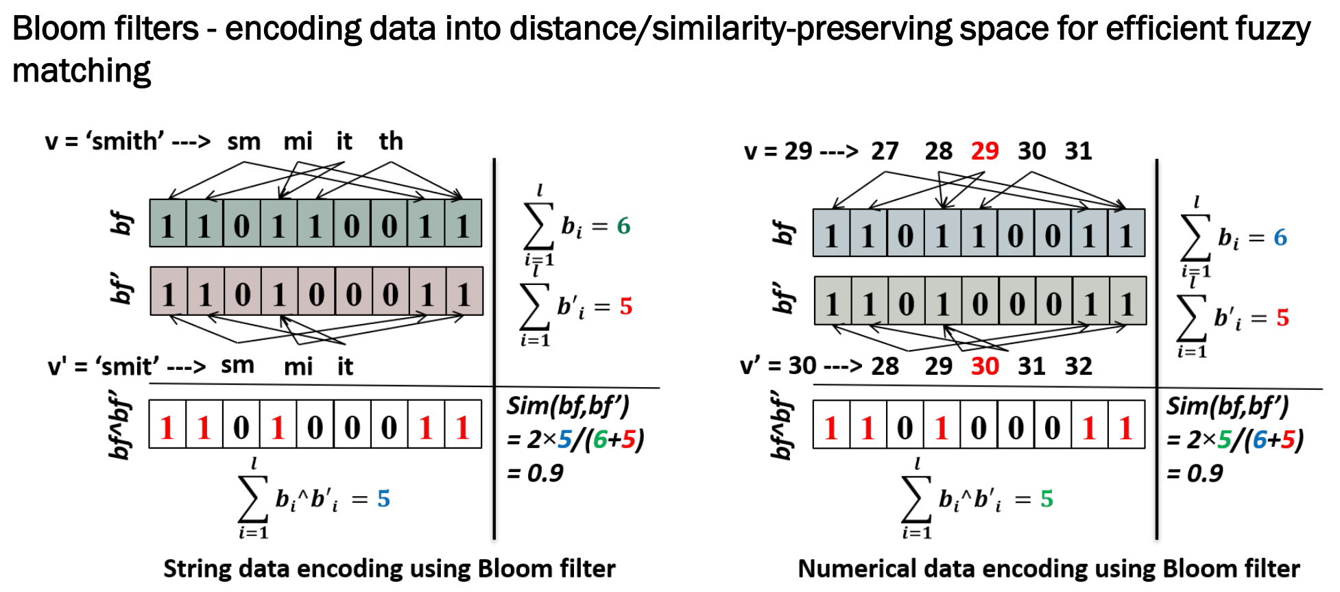
String Example: “smith” vs “smit”

Step 1: Break into bigrams

"smith" → sm, mi, it, th   (4 bigrams)
"smit"  → sm, mi, it       (3 bigrams, missing "th")

Step 2: Map into Bloom filters

bf  = 1 1 0 1 1 0 0 1 1   (6 bits set)
bf' = 1 1 0 1 0 0 0 1 1   (5 bits set)

Step 3: Calculate similarity

AND = 1 1 0 1 0 0 0 1 1   (5 matching bits)
Sim = 2 × 5 / (6 + 5) = 0.9  ✅ Very similar!

Numerical Example: 29 vs 30

Instead of bigrams, nearby values are generated to capture closeness:

v  = 29 → {27, 28, 29, 30, 31}
v' = 30 → {28, 29, 30, 31, 32}

Sim = 2 × 5 / (6 + 5) = 0.9  ✅ Very similar!

Key Difference from Exact Matching

	Exact Matching	Fuzzy Matching
“smith” vs “smit”	0.0 ❌	0.9 ✅
29 vs 30	0.0 ❌	0.9 ✅

Fuzzy matching is far more practical in real-world scenarios where typos, abbreviations, and minor errors are common.

---

Bloom Filters with Provable Privacy Guarantees

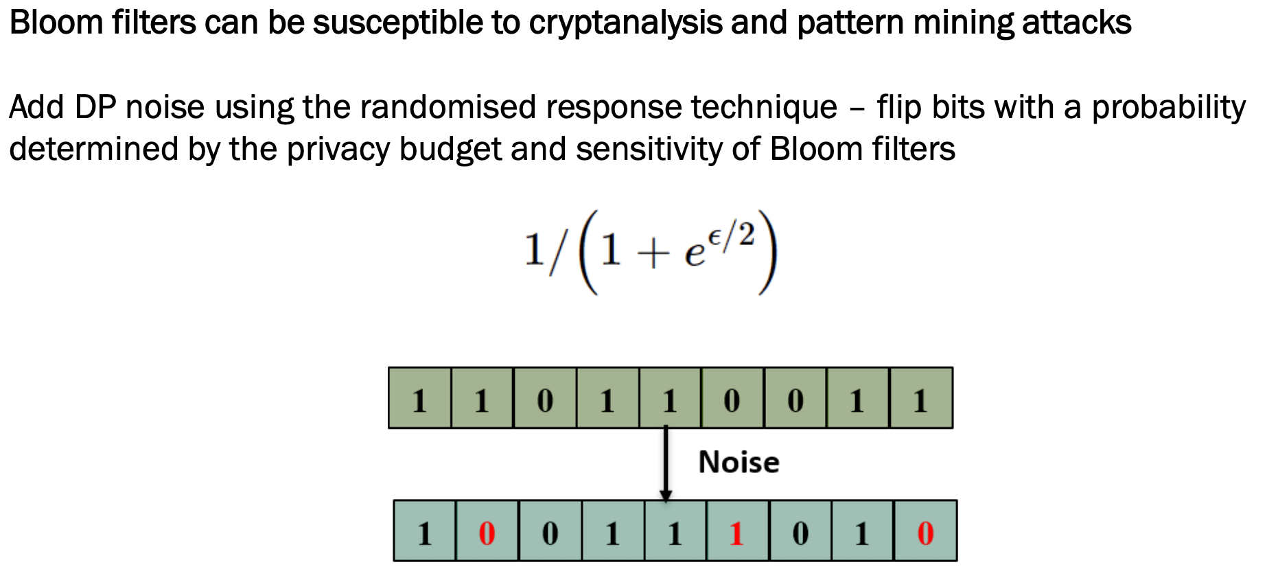
The Problem

Bloom filters alone are not fully secure. Attackers can potentially:

• Use cryptanalysis to reverse-engineer original data from the bit vector
• Use pattern mining to identify individuals by analysing repeated patterns

The Solution: Differential Privacy (DP) Noise

Random noise is added using Randomised Response — randomly flip some bits so attackers cannot fully trust what they see.

Original Bloom filter:

1  1  0  1  1  0  0  1  1

After adding noise (flipped bits):

1  0  0  1  1  1  0  1  0

The Flipping Probability Formula

\[p = \frac{1}{1 + e^{\varepsilon/2}}\]

Where ε (epsilon) is the privacy budget:

ε value	Flip probability	Privacy	Accuracy
Small ε	High (more flips)	Stronger 🔒	Lower
Large ε	Low (fewer flips)	Weaker	Higher ✅

This is the classic privacy vs accuracy trade-off in differential privacy.

Why Attackers Can’t Simply Reverse It

The attacker knows the formula, but NOT which bits were flipped, how many, or where. The flipping is random each time — even running the same name through twice gives different noisy outputs.

---

Text Data Encoding: Counting Bloom Filters (CBF)

Why a Different Approach for Text?

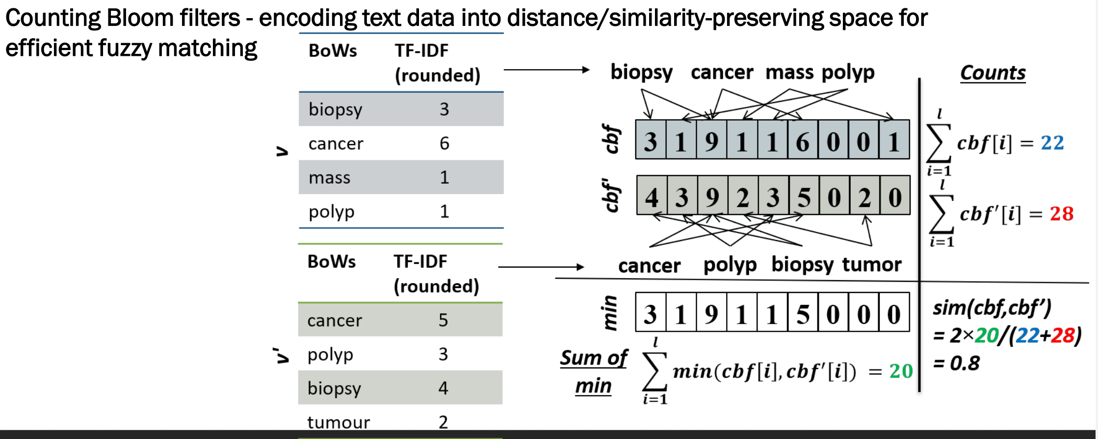
Regular Bloom filters just store 0s and 1s, which works for names and numbers. But for longer medical text, we need to capture how important each word is — not just whether it appears. That’s where Counting Bloom Filters (CBF) come in.

Step 1: TF-IDF Weighting

Record v	Score	Record v’	Score
biopsy	3	cancer	5
cancer	6	polyp	3
mass	1	biopsy	4
polyp	1	tumour	2

Step 2: Map into CBF

cbf  = 3 1 9 1 1 6 0 0 1   (total = 22)
cbf' = 4 3 9 2 3 5 0 2 0   (total = 28)

Step 3: Calculate Similarity

min  = 3 1 9 1 1 5 0 0 0   (sum of min = 20)
sim  = 2 × 20 / (22 + 28) = 0.8  ✅ Pretty similar!

A score of 0.8 correctly reflects that the two records share cancer, biopsy, and polyp but differ in “mass” vs “tumour” — very similar but not identical.

---

Matching and Linkage

Method	Pros	Cons
Threshold-based	Simple, fast	Hard to set the right threshold
Probabilistic (Fellegi-Sunter)	Accounts for errors	Needs prior error estimates
Rule-based (Deterministic)	Interpretable	Time consuming to build
ML-based	Flexible, accurate	Needs labelled training data

---

Evaluation

1. Computational Efficiency

Metric	What it measures
Runtime	How long it takes to run
Memory consumption	How much RAM is used
Communication size	How much data is sent between databases
Reduction ratio	How much blocking reduced comparisons
Pairs completeness	Whether blocking kept all true matches in same block

2. Linkage Quality

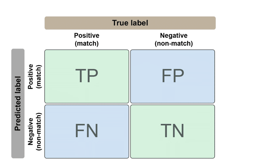
	Actually a Match	Actually NOT a Match
Predicted Match	TP (correct!)	FP (false alarm)
Predicted Non-match	FN (missed!)	TN (correct!)

\[\text{Accuracy} = \frac{TP + TN}{TP + FP + TN + FN}\] \[\text{Precision} = \frac{TP}{TP + FP}\] \[\text{Recall} = \frac{TP}{TP + FN}\] \[\text{F-measure} = \frac{2 \times Precision \times Recall}{Precision + Recall}\]

3. Privacy

Metric	What it measures
Entropy / information gain	How much info an attacker could extract
False positive rate of Bloom filter	How hard it is to reverse-engineer original data
Privacy budget (ε)	How much noise was added via differential privacy

---

Machine Learning: Attacks on ML Models

AI and ML models can be attacked in two main ways:

1. Inference Attacks

Membership Inference Attack — “Was this specific person’s data used to train this model?”

Attribute Inference Attack — “What are this person’s private attributes?” (uses the model to fill in missing info)

2. Adversarial Attacks

The attacker manipulates the input to trick the model into producing a desired (incorrect) output.

Attack type	Goal
Membership inference	Find out if a record was in the training data
Attribute inference	Infer private details about an individual
Adversarial	Manipulate the model’s output

---

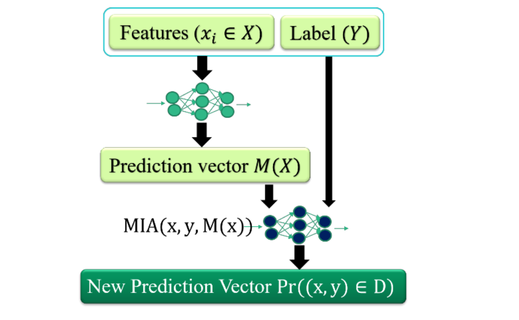
Membership Inference Attack (MIA)

Given a trained ML model and a record, determine whether that record was part of the model’s training data.

How it works

Features (x) + Label (y)  →  ML model  →  Prediction vector M(x)
                                                    ↓
                                          MIA(x, y, M(x))
                                                    ↓
                                   Pr((x,y) ∈ D)  →  Member or Not?

Why does this work?

Data type	Model behaviour
Training data (member)	Very high confidence, low loss
New data (non-member)	Lower confidence, higher loss

The attacker exploits this difference to distinguish members from non-members.

---

Black Box MIA

In a black box setting, the attacker can only send inputs and observe outputs — no access to model weights, architecture, or training data.

Three Levels of Information

Setting	Info available	Attack difficulty
Full confidence scores	All class scores	Easy
Top-k confidence scores	Partial scores	Moderate
Prediction label only	Just the label	Hard

Why We Can’t Always Use Label Only

Even with just a label, MIA is still possible (harder, but not impossible). More importantly, in PPRL you need to know how similar two records are — a binary “match / non-match” loses critical information.

Real Defences

• Differential privacy during training
• Output perturbation (adding noise to confidence scores)
• Restricting output detail (label only where possible)
• Limiting query rates

---

MIA against Text Linkage Model

	Detail
Input	Free-text mentor feedback (sequence of words)
Output	Categorical label (feedback classification)

Standard MIA definitions may not work well here — free-text input requires a looser/relaxed definition of MIA.

Three Black-box MIA Approaches

Attack	Method	Complexity
Shadow model (Shokri et al., 2017)	Trains multiple shadow models to mimic target	High
Prediction loss (Yeom et al., 2018)	Low loss → likely member	Moderate
Max confidence (Salem et al., 2018)	High confidence → likely member	Low

---

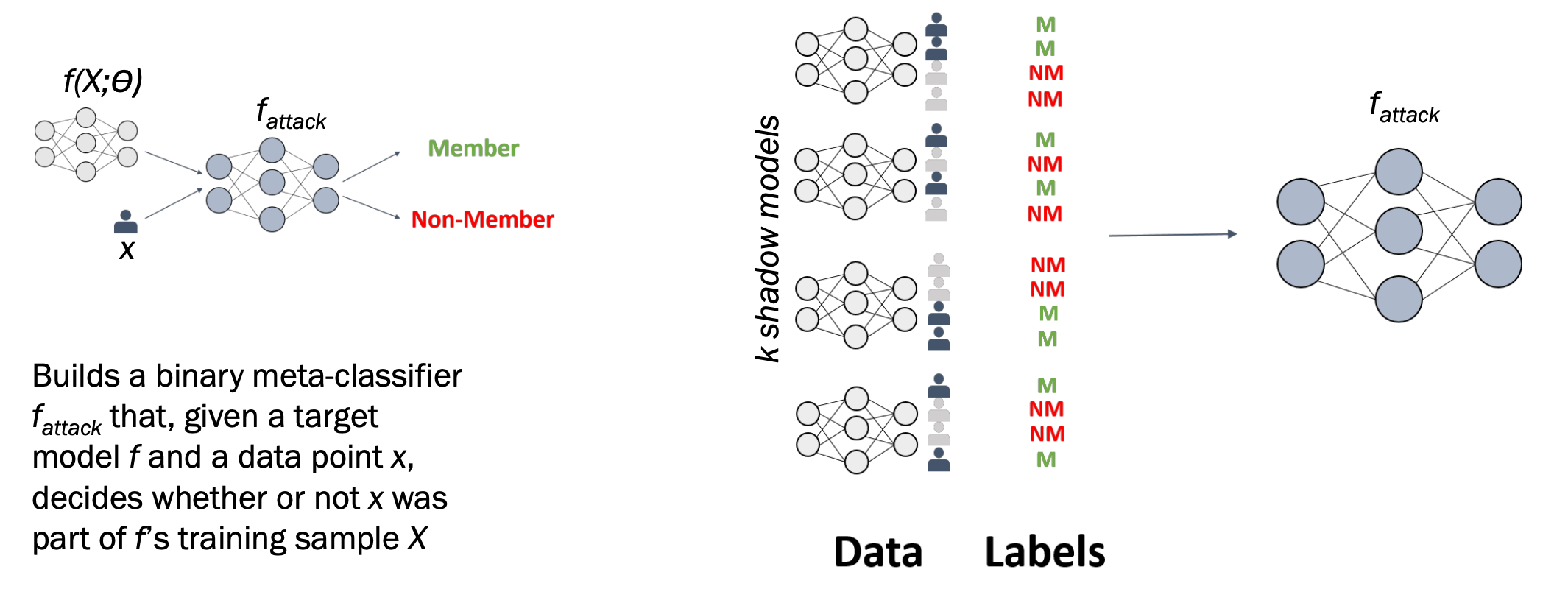
Shadow Model-based MIA

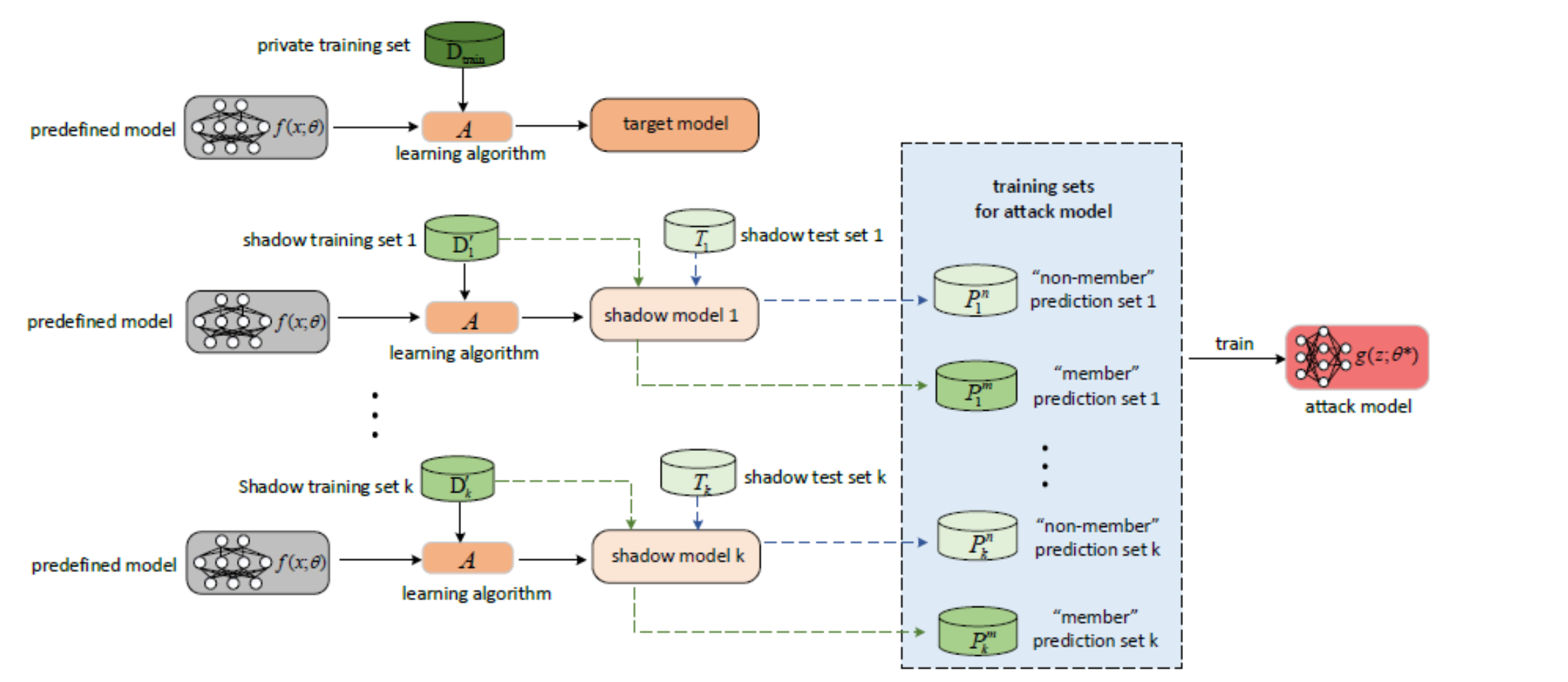
The attacker creates fake versions (shadow models) of the target model to learn how it behaves.

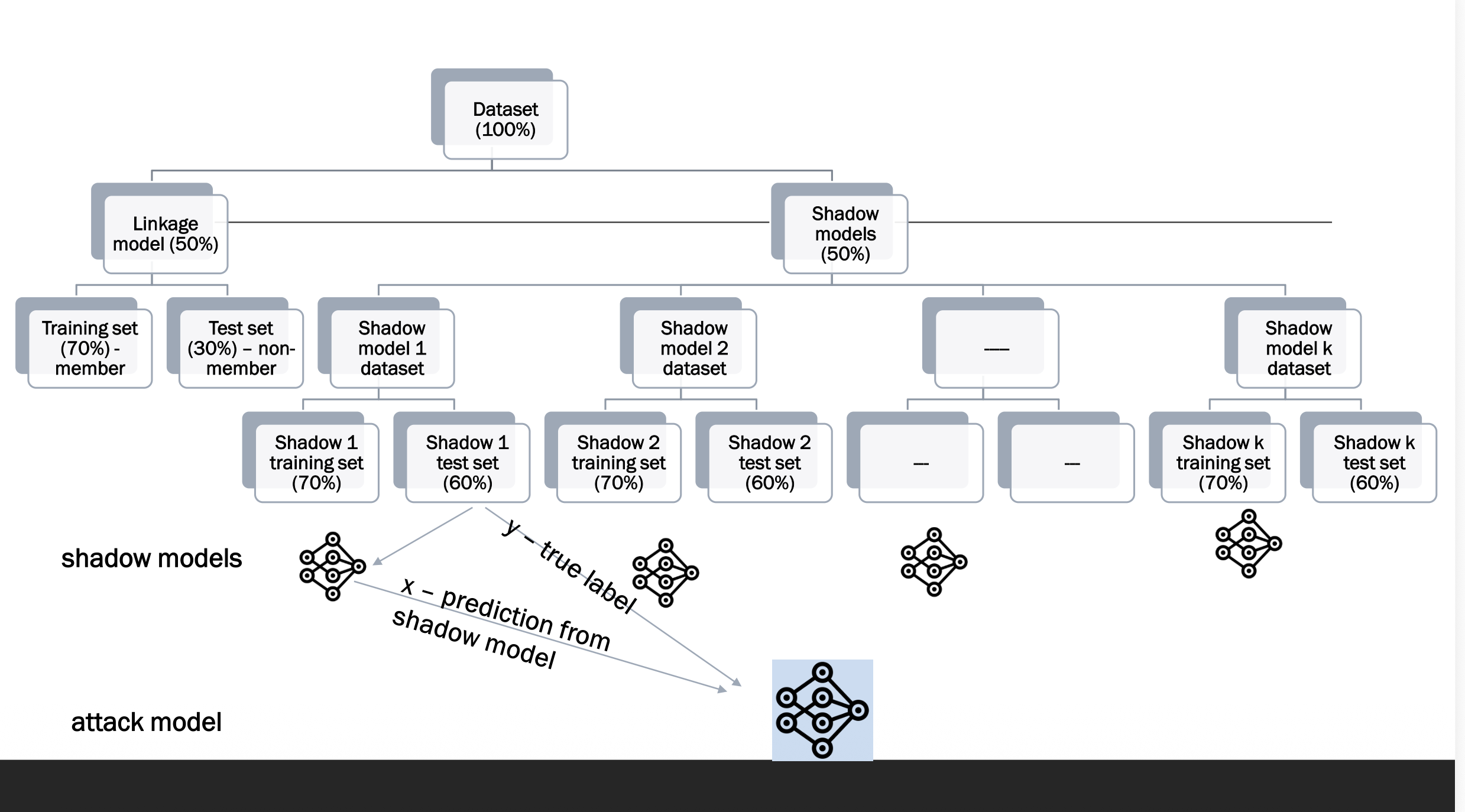
Step-by-Step

Step 1: Target model trained on private data D_min — the attacker cannot see inside it.

Step 2: Attacker trains k shadow models on similar but different data to mimic the target.

Step 3: For each shadow model, the attacker labels outputs as member (M) or non-member (NM).

Step 4: All labelled outputs train the attack model f_attack.

Shadow models learn to mimic target model
        ↓
Generate M / NM labelled predictions
        ↓
Train f_attack on those labels
        ↓
Apply f_attack to the real target model
        ↓
Determine: Member or Non-Member? 🔍

Analogy: Like practising on past exam papers to learn the examiner’s patterns, then applying that knowledge to the real exam.

---

Experiments: MIA with Standard Input Space (CIFAR-10)

Detail	Value
Dataset	CIFAR-10 image dataset
Data size	6,000 images, 10 classes
Image size	32×32 pixels (RGB)
Model	Logistic regression
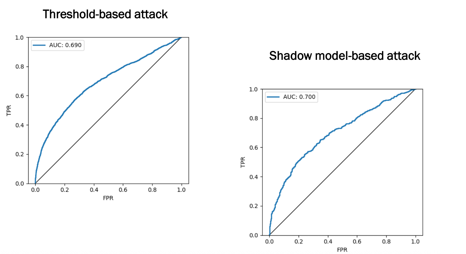
Attacks	Threshold-based + Shadow model-based

Attack	AUC
Threshold-based	0.690
Shadow model-based	0.700

Both attacks are meaningfully better than random guessing (AUC = 0.5), confirming that even a simple logistic regression on image data leaks membership information.

---

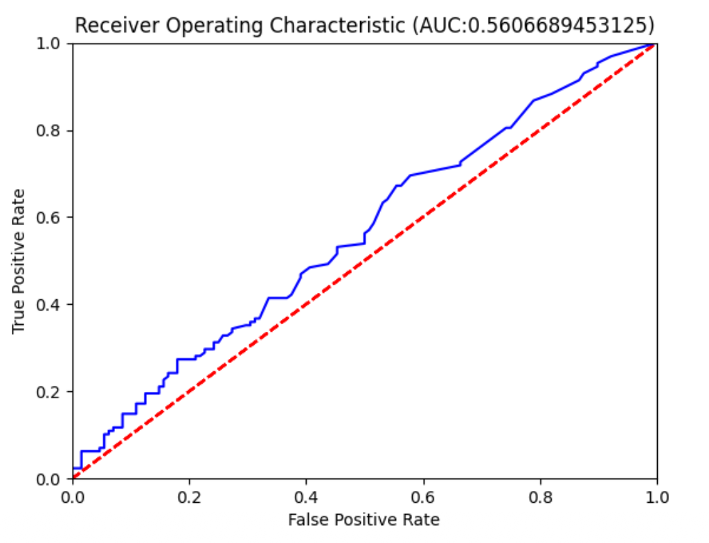
Experiments: MIA with Free-text Input Space

Detail	Value
Dataset	Free-text mentor feedback
Pre-processing	Remove stop words + lemmatise
Representation	Bag of Words (2,233 BoWs)
Labels	5 categories (outstanding → poor)
Model	Logistic regression

Result: AUC = 0.56 — barely better than random guessing.

Why is the AUC So Much Lower Than CIFAR-10?

1. High dimensionality — 2,233 sparse BoW features vs clean RGB pixels
2. More variability — people write feedback many different ways → less overfitting
3. 5 output classes — confidence scores more spread out, harder to exploit

Setting	Attack	AUC
CIFAR-10	Threshold	0.690
CIFAR-10	Shadow model	0.700
Free-text (large)	Shadow model	0.560

---

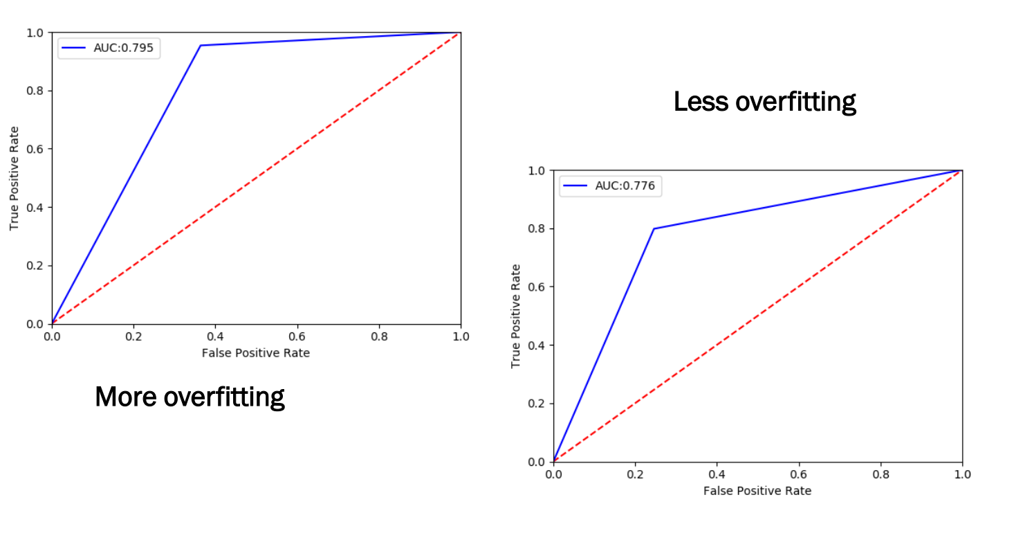
Experiments: Free-text MIA (Small Dataset, Overfitting)

Detail	Value
Dataset	Small free-text feedback (1,633 BoWs)
Model	ANN classifier

Setting	AUC
More overfitting	0.795
Less overfitting	0.776

Why Does Overfitting Make MIA Easier?

Overfitted model:
  Members   →  Very high confidence, very low loss
  Non-members →  Much lower confidence, higher loss

More overfitting  →  Bigger gap  →  AUC 0.795 (easier to attack)
Less overfitting  →  Smaller gap →  AUC 0.776 (slightly harder)

Reducing overfitting (regularisation, dropout, early stopping) is an effective privacy defence as well as good ML practice!

---

Experiments: Free-text MIA (Multiple Shadow Models)

Number of shadow models	AUC
10 shadow models	0.776
5 shadow models	0.747

More shadow models → more diverse training data for the attack model → higher AUC.

Full Summary of Free-text Experiments

Setting	AUC
Large dataset, logistic regression	0.560
Small dataset, less overfitting, 10 shadow models	0.776
Small dataset, more overfitting, 10 shadow models	0.795
Small dataset, less overfitting, 5 shadow models	0.747

Three Key Factors That Increase MIA Vulnerability

1. Smaller dataset → more overfitting → easier to attack
2. More overfitting → bigger gap between member/non-member behaviour → easier to attack
3. More shadow models → better trained attack model → easier to attack